Imagine trying to photograph a single layer inside a dense forest without capturing the treetops above or roots below. That’s the challenge biologists face when imaging thick biological samples. In conventional microscopes, out-of-focus light blurs the target plane, obscuring fine details. But with a confocal microscope, researchers can isolate a razor-thin optical section—revealing crisp, high-contrast images of subcellular structures in 3D.
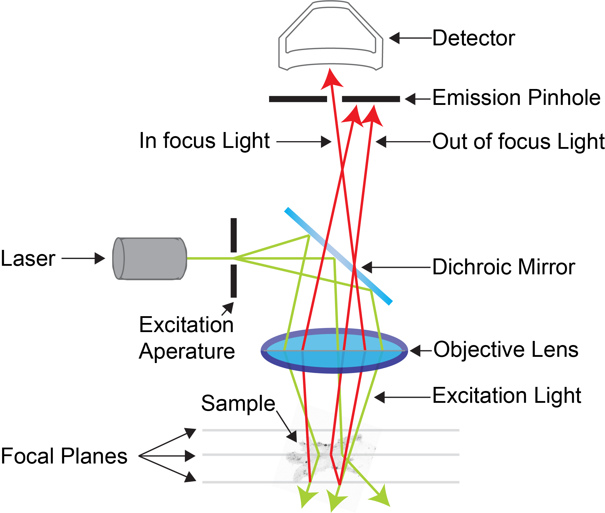
At its core, a confocal microscope works by eliminating out-of-focus fluorescence using a smart optical trick: the confocal pinhole. Unlike widefield microscopes that illuminate the entire sample at once, confocal systems scan a focused laser point-by-point across the specimen. Only light emitted precisely from the focal plane passes through the pinhole to reach the detector. Light from above or below is blocked, dramatically improving clarity and enabling 3D reconstructions of complex tissues, cells, and materials.
You’ll discover how lasers, scanning mirrors, dichroic mirrors, and precision apertures work in concert to achieve optical sectioning. We’ll break down the full light path, compare major confocal types (laser scanning vs. spinning disk), and explore real-world applications from neuroscience to cancer research. By the end, you’ll understand not just how it works—but why it’s a cornerstone of modern imaging.
Core Principle: Optical Sectioning Explained
The magic of confocal microscopy lies in its ability to generate clear images from within thick specimens—without physically slicing them. This is called optical sectioning, and it’s made possible by a simple but powerful design: alignment of two focal points.
What Makes It “Confocal”?
“Confocal” means two shared focal points in the optical system:
– One at the sample plane (under the objective lens)
– One at the detection pinhole
These points lie in conjugate planes, meaning light that comes into focus at the sample is also focused exactly onto the pinhole. Only in-focus light passes through; everything else gets rejected.
How the Pinhole Blocks Blur
When the laser hits the sample, fluorophores emit light—not just in the plane you want, but above and below too. In widefield microscopy, all this light reaches the camera, creating haze. But in a confocal:
– In-focus light converges perfectly on the pinhole → passes through
– Out-of-focus light arrives divergent → blocked by the aperture
This selective filtering slashes background noise and sharpens both lateral (XY) and axial (Z) resolution. Axial resolution improves from ~1 µm in widefield to ~0.5 µm in confocal—critical for 3D imaging.
Pinhole Size: Balancing Signal and Clarity
The pinhole diameter is typically set around 1 Airy unit (AU)—the size of the diffraction-limited spot produced by a perfect lens.
– Smaller than 1 AU: Sharper sections, higher contrast—but dimmer signal
– Larger than 1 AU: Brighter image, but more out-of-focus light sneaks through
Modern systems let users adjust the pinhole in real time, optimizing for resolution or sensitivity depending on the sample.
Laser Scanning Light Path Breakdown
A confocal microscope doesn’t take a snapshot—it builds an image pixel by pixel using a scanning laser. Here’s how each component directs light to create a sharp, optical slice.
Laser Source: Precision Excitation
Confocal microscopes use lasers instead of lamps because they deliver:
– High intensity
– Monochromatic (single-wavelength) light
– Tight beam collimation
Common lasers include:
– 405 nm (violet): For DAPI and Hoechst nuclear stains
– 488 nm (blue): Excites GFP, fluorescein
– 561 nm (yellow-green): For RFP, mCherry
– 633 nm (red): For far-red dyes like Cy5
Multiple lasers allow multicolor imaging, letting researchers label and distinguish different structures in one sample.
Dichroic Mirror: Wavelength Traffic Director
This specialized mirror acts like a one-way gate based on wavelength:
– Reflects short-wavelength excitation light toward the sample
– Transmits long-wavelength emitted fluorescence to the detector
For example, a 488/561 dichroic reflects blue and green lasers but lets yellow, red, and far-red emission pass. Often, multiple dichroics are used in tandem for multi-laser setups.
Emission filters after the mirror further refine the signal, blocking any stray laser light and isolating the desired emission band (e.g., 500–550 nm for GFP).
Scanning Mirrors: Steering the Laser Dot
Two galvanometer-controlled mirrors raster-scan the laser across the sample:
– X-mirror: Horizontal movement
– Y-mirror: Vertical movement
They move in sync to illuminate each point in a grid pattern—like reading lines of text. A typical 512×512 image requires over 260,000 individual measurements.
Advanced systems use acousto-optic deflectors (AODs) for even faster scanning—up to hundreds of frames per second—ideal for live-cell dynamics.
Objective Lens: Focus and Collection Power
High numerical aperture (NA) objectives (e.g., 1.4 NA oil immersion) do two things:
– Tightly focus the laser into a diffraction-limited spot
– Efficiently collect emitted photons
The NA determines resolution and light-gathering ability—higher NA = sharper, brighter images.
Confocal Pinhole: The Gatekeeper
Located at a conjugate plane to the focal point, the pinhole ensures only in-focus light reaches the detector. Some systems offer adjustable pinholes; others use fixed sizes matched to specific objectives.
If the pinhole is misaligned—even slightly—image quality drops fast. Proper alignment is essential for optimal performance.
Detector: Capturing Single Photons
Because only a tiny spot emits light at any moment, detectors must be extremely sensitive:
– Photomultiplier Tubes (PMTs): Amplify weak signals via electron multiplication; ideal for low-light scanning
– Avalanche Photodiodes (APDs): More efficient in near-infrared range
– Hybrid Detectors (HyDs): Combine speed, linearity, and dynamic range
Detectors convert photons into electrical signals, which are digitized and stored as pixel intensities.
Image Formation: Building Pixel by Pixel
There’s no direct image formation on a sensor. Instead:
1. The detector records intensity at each scanned point
2. The computer maps that value to a pixel based on mirror position
3. After scanning all points, a full 2D image appears on screen
This sequential process enables precise control—but limits speed compared to camera-based systems.
3D Imaging with Z-Stacks
One of the biggest advantages of confocal microscopy is 3D reconstruction of biological structures. You can’t see depth in a single 2D image—but by capturing multiple slices, you can.
Acquiring Optical Sections
To build a 3D volume:
1. Focus on the top of your sample
2. Capture an image
3. Move the stage (or objective) down slightly (e.g., 0.2 µm)
4. Repeat until you’ve imaged through the entire specimen
This series of images is called a Z-stack. Step size depends on required resolution and sample thickness—typically 0.1 to 1.0 µm.
Reconstructing 3D Volumes
Software combines Z-stacks into 3D models using techniques like:
– Maximum Intensity Projection (MIP): Shows brightest pixel along each line of sight
– Volume Rendering: Assigns color/opacity to different intensity levels
– Surface Rendering: Creates mesh models of structures (e.g., mitochondria)
These reconstructions reveal spatial relationships—like how neurons connect in brain tissue or how tumor cells invade surrounding stroma.
Applications of 3D Analysis
Researchers use Z-stacks to:
– Measure organelle volume changes during apoptosis
– Track cell migration in developing embryos
– Quantify co-localization of proteins in 3D space
– Visualize vascular networks in tumors
Without physical sectioning, confocal Z-stacking preserves sample integrity while delivering detailed volumetric data.
Confocal vs. Widefield: Why Contrast Matters
While both use fluorescence, confocal and widefield microscopes produce very different results—especially in thick samples.
Widefield Limitations
In widefield:
– Entire sample illuminated at once
– All emitted light collected—including out-of-focus blur
– Results in hazy, low-contrast images
Even with deconvolution software, widefield struggles with samples thicker than ~20 µm.
Confocal Advantages
By rejecting out-of-focus light, confocal:
– Boosts image contrast dramatically
– Improves signal-to-noise ratio
– Enables optical sectioning in samples up to 100 µm thick
– Reduces background for more accurate quantification
For example, imaging a fluorescently labeled nucleus deep in a tissue section:
– Widefield: Glow spreads above and below, making edges fuzzy
– Confocal: Crisp boundary, clean background
This clarity makes confocal essential for precise localization and 3D analysis.
Types of Confocal Microscopes
Not all confocals work the same way. Different designs balance speed, resolution, and phototoxicity for specific applications.
Laser Scanning Confocal (LSCM)
Also called point-scanning confocal, this is the most common type.
How It Works
- Single laser spot scanned across sample
- Light descanned through same mirrors
- Passes through pinhole → detected by PMT
Pros
- Best resolution and optical sectioning
- Ideal for thick, fixed samples
- Full control over scanning parameters
Cons
- Slower acquisition (1–30 fps)
- Higher photobleaching risk in live samples
Best For
- High-resolution 3D imaging
- Immunofluorescence
- Subcellular structure analysis
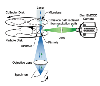
Spinning Disk Confocal
Uses a rotating disk with thousands of microlens-pinhole pairs for parallel scanning.
How It Works
- Disk spins rapidly (5,000+ rpm)
- Microlenses focus light onto pinholes
- Multiple points illuminated simultaneously
- Emitted light captured by sCMOS or EM-CCD camera
Pros
- Much faster (up to 1,000 fps)
- Lower laser power → less photodamage
- Great for live-cell imaging
Cons
- Lower Z-resolution due to pinhole crosstalk
- Less flexible pinhole adjustment
- Not ideal for very thick samples
Best For
- Calcium signaling
- Mitosis tracking
- Zebrafish embryo development
Hybrid Scanning Systems
Combine laser scanning and spinning disk in one platform.
Features
- Switch between modes as needed
- Use point scanning for high-res static images
- Use multi-point for fast time-lapse
Advantages
- Flexibility for diverse experiments
- Optimized workflows for long-term studies
Best For
- High-throughput screening
- Dual-mode imaging (static + dynamic)
Fluorescence Fundamentals Recap
To fully grasp confocal imaging, it helps to understand how fluorophores behave.
Excitation and Emission
Fluorophores absorb high-energy (short-wavelength) light and emit lower-energy (longer-wavelength) light. This shift is called the Stokes shift.
Example:
– GFP excited at 488 nm → emits at ~510 nm (green)
– Emission filter blocks 488 nm laser light, allowing only green to pass
This spectral separation allows clean signal detection.
Common Fluorophores
| Fluorophore | Excitation (nm) | Emission (nm) | Color |
|---|---|---|---|
| DAPI | 358 | 461 | Blue |
| FITC | 495 | 519 | Green |
| TRITC | 557 | 576 | Orange |
| Cy5 | 650 | 670 | Red |
Genetically encoded proteins like GFP, mCherry, YFP let researchers tag specific proteins in living cells—revolutionizing cell biology.
Multicolor Imaging
By using multiple lasers and filters, confocals can image several fluorophores at once. Channels are acquired sequentially to avoid bleed-through, then merged digitally.
This allows studies of:
– Protein-protein interactions
– Organelle dynamics
– Gene expression patterns
Step-by-Step: How It All Comes Together
Let’s walk through the full imaging cycle—from laser to final image.
1. Laser Emission
A 488 nm laser fires a beam of blue light into the system.
2. Beam Steering
The dichroic mirror reflects the laser toward the scanning mirrors.
3. Sample Scanning
Galvanometer mirrors raster-scan the focused beam across the sample, illuminating one spot at a time.
4. Fluorescence Emission
GFP-labeled proteins in the focal plane absorb blue light and emit green fluorescence.
5. Light Return Path
Emission travels back through the objective, passes through the dichroic (now transparent to green), and retraces the path through scanning mirrors (descanning).
6. Pinhole Filtering
Light converges at the confocal pinhole. Only in-focus photons pass through; out-of-focus light is blocked.
7. Detection
PMT detects the green signal, converting photons into an electrical current.
8. Pixel Mapping
Computer records intensity and assigns it to a pixel based on mirror position.
9. Image Assembly
After scanning all points, a 512×512 image forms—pixel by pixel.
10. 3D Volume Build
Stage moves down 0.2 µm. Process repeats. After 50 slices, software stacks them into a 3D model.
Practical Considerations and Trade-offs
Confocal microscopy delivers exceptional images—but comes with challenges.
Photobleaching and Phototoxicity
Even with optical sectioning, prolonged laser exposure damages fluorophores and live cells.
Solutions:
– Use lowest laser power needed
– Reduce pixel dwell time
– Add oxygen scavengers (e.g., OxyFluor)
– Use sensitive detectors to minimize excitation
Spinning disk systems are gentler for long-term live imaging.
Sample Preparation Tips
- Use anti-fade mounting media (e.g., ProLong Diamond)
- Optimize antibody concentrations to reduce background
- Choose fluorophores with high quantum yield and photostability
- Match immersion medium (oil, water, glycerol) to objective
System Complexity
Confocals require:
– Regular alignment checks
– Calibration of lasers and detectors
– Expertise in acquisition settings (gain, offset, Z-step)
Training and maintenance are key to consistent results.
Cost Factor
High-end confocals cost $300,000–$600,000 due to:
– Multiple lasers
– Precision optics
– Sensitive detectors
– Vibration-isolated stages
Core facilities often house these systems for shared access.
Real-World Applications
Confocal microscopy isn’t just for pretty pictures—it drives discovery across science.
Cell Biology
Visualize:
– Mitochondrial fission/fusion
– Lysosome movement
– Actin cytoskeleton remodeling
– Nuclear envelope breakdown during mitosis
Use FRAP (Fluorescence Recovery After Photobleaching) to study protein mobility.
Neuroscience
Map:
– Dendritic spines
– Synaptic connections
– Axonal transport
– Amyloid plaques in Alzheimer’s models
3D imaging reveals neural circuitry in brain slices.
Cancer Research
Analyze:
– Tumor spheroid structure
– Angiogenesis
– Cell invasion into matrix
– Drug penetration and efficacy
Co-localization studies show protein interactions in cancer pathways.
Developmental Biology
Image live:
– Zebrafish embryogenesis
– Drosophila segmentation
– Organ formation in mouse embryos
Time-lapse confocal captures dynamic morphogenetic events.
Materials Science
Study:
– Polymer phase separation
– Composite material interfaces
– Nanoparticle distribution
– Microcrack propagation
Fluorescent tags reveal internal structure without destruction.
Historical Milestones
- 1957: Marvin Minsky patents the confocal principle—using a pinhole to reject out-of-focus light
- 1960s: Invention of the laser enables practical implementation
- 1970s: First functional confocal built (by Egger and Petran)
- 1980s–90s: Commercial systems emerge (e.g., Bio-Rad, Zeiss)
- 2000s–present: Spinning disk, hybrid systems, and super-resolution extensions evolve
Minsky’s original design moved the sample; modern versions scan the light—faster and more precise.
Final Note: Confocal microscopy transforms how we see the microscopic world. By combining laser precision, optical filtering, and computational imaging, it delivers clarity unattainable with conventional methods. Whether you’re studying synaptic vesicles in neurons or drug diffusion in tumors, understanding how a confocal microscope works empowers better experimental design, sharper images, and deeper insights.